![]()
![]()
![]()
![]()
![]()
The goal of mvgam is to fit Bayesian Dynamic Generalized Additive Models to time series data. The motivation for the package is described in Clark & Wells 2022 (published in Methods in Ecology and Evolution), with additional inspiration on the use of Bayesian probabilistic modelling coming from Michael Betancourt, Michael Dietze and Emily Fox, among many others.
A series of vignettes cover data formatting, forecasting and several extended case studies of DGAMs. A number of other examples have also been compiled:
mgcv and mvgamInstall the stable version from CRAN using: install.packages('mvgam'), or install the development version from GitHub using: devtools::install_github("nicholasjclark/mvgam"). Note that to condition models on observed data, either JAGS (along with packages rjags and runjags) or Stan must be installed (along with either rstan and/or cmdstanr). Please refer to installation links for JAGS here, for Stan with rstan here, or for Stan with cmdstandr here. You will need a fairly recent version of Stan to ensure all syntax is recognized. If you see warnings such as variable "array" does not exist, this is usually a sign that you need to update Stan. We highly recommend you use Cmdstan through the cmdstanr interface. This is because Cmdstan is easier to install, is more up to date with new features, and uses less memory than Rstan. See this documentation from the Cmdstan team for more information.
When using any software please make sure to appropriately acknowledge the hard work that developers and maintainers put into making these packages available. Citations are currently the best way to formally acknowledge this work, so we highly encourage you to cite any packages that you rely on for your research.
When using mvgam, please cite the following:
As mvgam acts as an interface to Stan and JAGS, please additionally cite whichever software you use for parameter estimation:
mvgam relies on several other R packages and, of course, on R itself. To find out how to cite R and its packages, use the citation function. There are some features of mvgam which specifically rely on certain packages. The most important of these is the generation of data necessary to estimate smoothing splines, which entirely rely on mgcv. The rstan and cmdstanr packages together with Rcpp makes Stan conveniently accessible in R, while the rjags and runjags packages together with the coda package make JAGS accessible in R. If you use some of these features, please also consider citing the related packages.

We can explore the model’s primary functions using a dataset that is available with all R installations. Load the lynx data and plot the series as well as its autocorrelation function
data(lynx)
lynx_full <- data.frame(year = 1821:1934,
                        population = as.numeric(lynx))
plot(lynx_full$population, type = 'l', ylab = 'Lynx trappings',
     xlab = 'Time', bty = 'l', lwd = 2)
box(bty = 'l', lwd  = 2)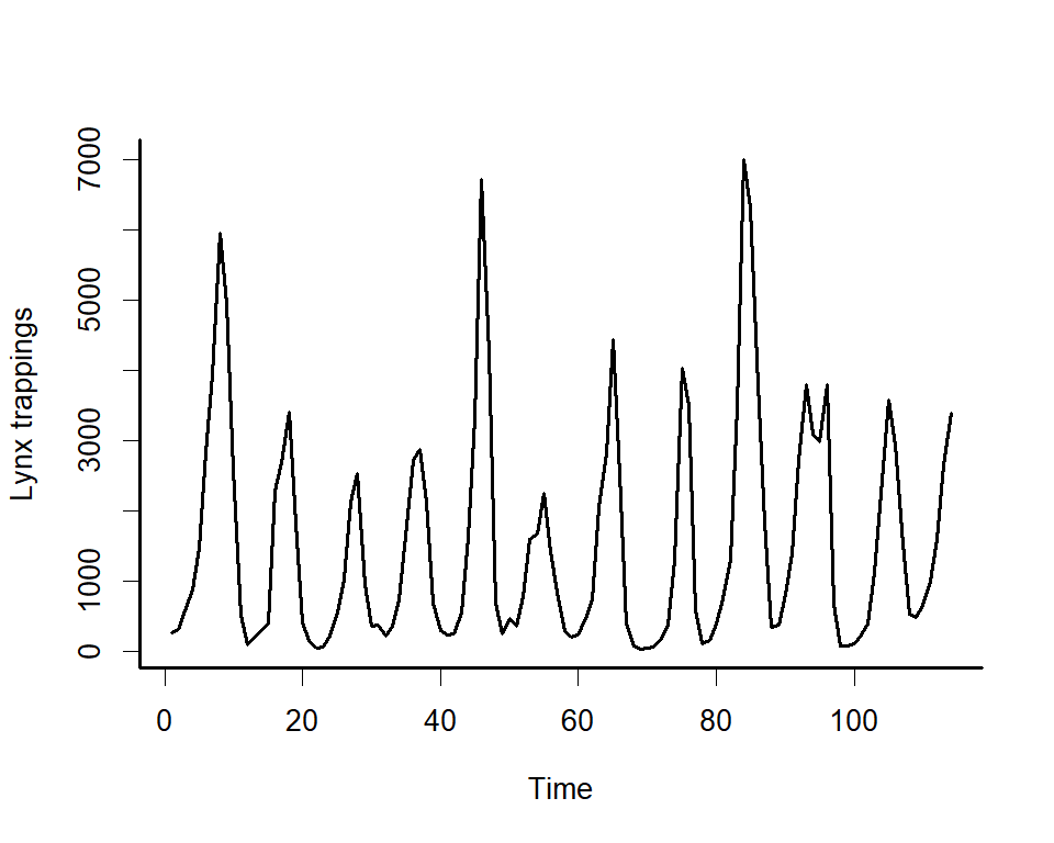
acf(lynx_full$population, main = '', bty = 'l', lwd = 2,
    ci.col = 'darkred')
box(bty = 'l', lwd  = 2)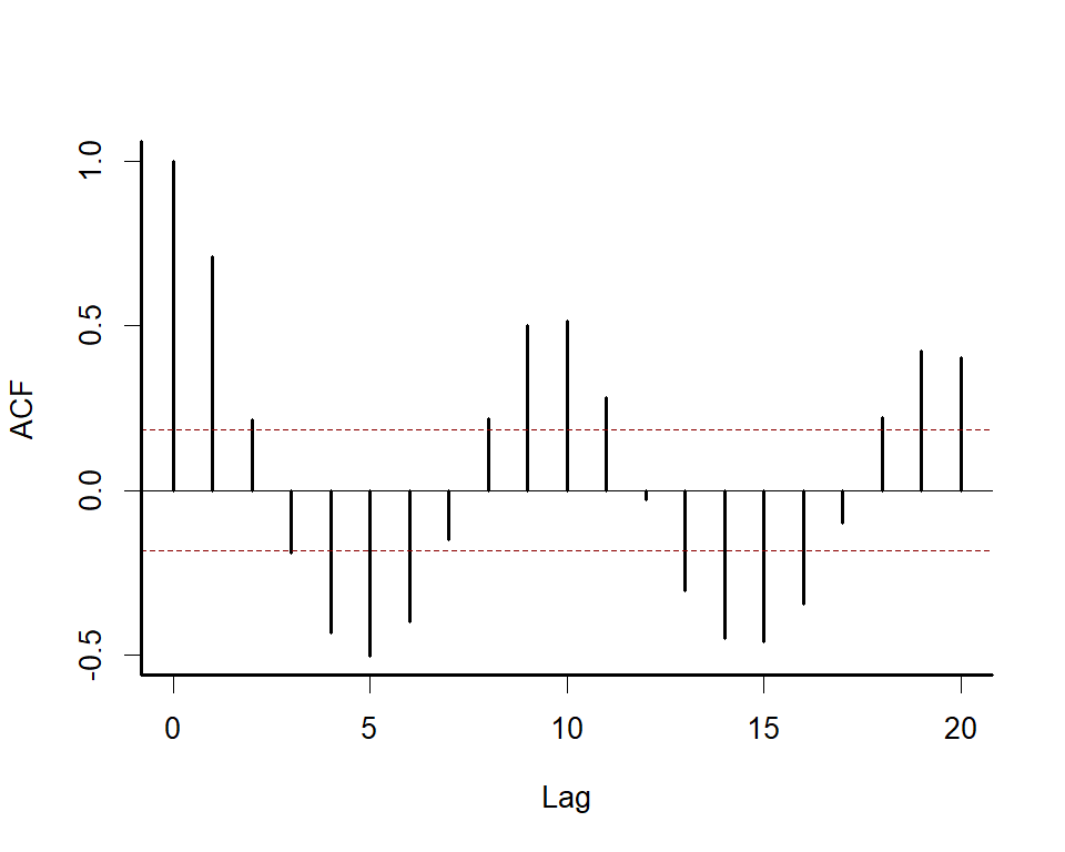
Along with serial autocorrelation, there is a clear ~19-year cyclic pattern. Create a season term that can be used to model this effect and give a better representation of the data generating process than we would likely get with a linear model
plot(stl(ts(lynx_full$population, frequency = 19), s.window = 'periodic'),
     lwd = 2, col.range = 'darkred')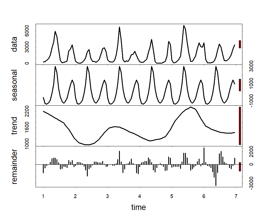
For mvgam models, we need an indicator of the series name as a factor (if the column series is missing, this will be added automatically by assuming that all observations are from a single time series). A time column is needed to index time
Split the data into training (first 50 years) and testing (next 10 years of data) to evaluate forecasts
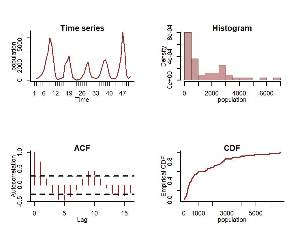
Inspect the series in a bit more detail using mvgam’s plotting utility
Now we will formulate an mvgam model; this model fits a GAM in which a cyclic smooth function for season is estimated jointly with a full time series model for the temporal process (in this case an AR3 process). We assume the outcome follows a Poisson distribution and will condition the model in Stan using MCMC sampling with the Cmdstan interface:
lynx_mvgam <- mvgam(population ~ s(season, bs = 'cc', k = 12),
                    knots = list(season = c(0.5, 19.5)),
                    data = lynx_train,
                    newdata = lynx_test,
                    family = poisson(),
                    trend_model = AR(p = 3),
                    backend = 'cmdstanr')
Inspect the Stan code for the model
code(lynx_mvgam)
#> // Stan model code generated by package mvgam
#> data {
#>   int<lower=0> total_obs; // total number of observations
#>   int<lower=0> n; // number of timepoints per series
#>   int<lower=0> n_sp; // number of smoothing parameters
#>   int<lower=0> n_series; // number of series
#>   int<lower=0> num_basis; // total number of basis coefficients
#>   vector[num_basis] zero; // prior locations for basis coefficients
#>   matrix[total_obs, num_basis] X; // mgcv GAM design matrix
#>   array[n, n_series] int<lower=0> ytimes; // time-ordered matrix (which col in X belongs to each [time, series] observation?)
#>   matrix[10, 10] S1; // mgcv smooth penalty matrix S1
#>   int<lower=0> n_nonmissing; // number of nonmissing observations
#>   array[n_nonmissing] int<lower=0> flat_ys; // flattened nonmissing observations
#>   matrix[n_nonmissing, num_basis] flat_xs; // X values for nonmissing observations
#>   array[n_nonmissing] int<lower=0> obs_ind; // indices of nonmissing observations
#> }
#> parameters {
#>   // raw basis coefficients
#>   vector[num_basis] b_raw;
#>
#>   // latent trend AR1 terms
#>   vector<lower=-1.5, upper=1.5>[n_series] ar1;
#>
#>   // latent trend AR2 terms
#>   vector<lower=-1.5, upper=1.5>[n_series] ar2;
#>
#>   // latent trend AR3 terms
#>   vector<lower=-1.5, upper=1.5>[n_series] ar3;
#>
#>   // latent trend variance parameters
#>   vector<lower=0>[n_series] sigma;
#>
#>   // latent trends
#>   matrix[n, n_series] trend;
#>
#>   // smoothing parameters
#>   vector<lower=0>[n_sp] lambda;
#> }
#> transformed parameters {
#>   // basis coefficients
#>   vector[num_basis] b;
#>   b[1 : num_basis] = b_raw[1 : num_basis];
#> }
#> model {
#>   // prior for (Intercept)...
#>   b_raw[1] ~ student_t(3, 6.5, 2.5);
#>
#>   // prior for s(season)...
#>   b_raw[2 : 11] ~ multi_normal_prec(zero[2 : 11],
#>                                     S1[1 : 10, 1 : 10] * lambda[1]);
#>
#>   // priors for AR parameters
#>   ar1 ~ std_normal();
#>   ar2 ~ std_normal();
#>   ar3 ~ std_normal();
#>
#>   // priors for smoothing parameters
#>   lambda ~ normal(5, 30);
#>
#>   // priors for latent trend variance parameters
#>   sigma ~ student_t(3, 0, 2.5);
#>
#>   // trend estimates
#>   trend[1, 1 : n_series] ~ normal(0, sigma);
#>   trend[2, 1 : n_series] ~ normal(trend[1, 1 : n_series] * ar1, sigma);
#>   trend[3, 1 : n_series] ~ normal(trend[2, 1 : n_series] * ar1
#>                                   + trend[1, 1 : n_series] * ar2, sigma);
#>   for (s in 1 : n_series) {
#>     trend[4 : n, s] ~ normal(ar1[s] * trend[3 : (n - 1), s]
#>                              + ar2[s] * trend[2 : (n - 2), s]
#>                              + ar3[s] * trend[1 : (n - 3), s], sigma[s]);
#>   }
#>   {
#>     // likelihood functions
#>     vector[n_nonmissing] flat_trends;
#>     flat_trends = to_vector(trend)[obs_ind];
#>     flat_ys ~ poisson_log_glm(append_col(flat_xs, flat_trends), 0.0,
#>                               append_row(b, 1.0));
#>   }
#> }
#> generated quantities {
#>   vector[total_obs] eta;
#>   matrix[n, n_series] mus;
#>   vector[n_sp] rho;
#>   vector[n_series] tau;
#>   array[n, n_series] int ypred;
#>   rho = log(lambda);
#>   for (s in 1 : n_series) {
#>     tau[s] = pow(sigma[s], -2.0);
#>   }
#>
#>   // posterior predictions
#>   eta = X * b;
#>   for (s in 1 : n_series) {
#>     mus[1 : n, s] = eta[ytimes[1 : n, s]] + trend[1 : n, s];
#>     ypred[1 : n, s] = poisson_log_rng(mus[1 : n, s]);
#>   }
#> }
Have a look at this model’s summary to see what is being estimated. Note that no pathological behaviours have been detected and we achieve good effective sample sizes / mixing for all parameters
summary(lynx_mvgam)
#> GAM formula:
#> population ~ s(season, bs = "cc", k = 12)
#>
#> Family:
#> poisson
#>
#> Link function:
#> log
#>
#> Trend model:
#> AR(p = 3)
#>
#> N series:
#> 1
#>
#> N timepoints:
#> 60
#>
#> Status:
#> Fitted using Stan
#> 4 chains, each with iter = 1000; warmup = 500; thin = 1
#> Total post-warmup draws = 2000
#>
#>
#> GAM coefficient (beta) estimates:
#>                 2.5%     50%  97.5% Rhat n_eff
#> (Intercept)   6.0000  6.6000  7.000 1.01   793
#> s(season).1  -0.6000  0.0570  0.740 1.00   899
#> s(season).2  -0.2500  0.7600  1.900 1.01   433
#> s(season).3   0.0054  1.1000  2.500 1.01   401
#> s(season).4  -0.5200  0.4200  1.400 1.00   934
#> s(season).5  -1.2000 -0.1500  0.980 1.01   542
#> s(season).6  -1.1000  0.0061  1.100 1.00   656
#> s(season).7  -0.8100  0.3300  1.400 1.01   887
#> s(season).8  -0.9800  0.1700  1.800 1.01   457
#> s(season).9  -1.1000 -0.3200  0.680 1.01   540
#> s(season).10 -1.4000 -0.6400 -0.027 1.01   746
#>
#> Approximate significance of GAM smooths:
#>            edf Ref.df Chi.sq p-value
#> s(season) 9.97     10  17566     0.3
#>
#> Latent trend AR parameter estimates:
#>           2.5%   50% 97.5% Rhat n_eff
#> ar1[1]    0.77  1.10 1.400 1.00   899
#> ar2[1]   -0.85 -0.40 0.038 1.00  1686
#> ar3[1]   -0.48 -0.13 0.300 1.01   562
#> sigma[1]  0.40  0.50 0.640 1.00  1202
#>
#> Stan MCMC diagnostics:
#> n_eff / iter looks reasonable for all parameters
#> Rhat looks reasonable for all parameters
#> 0 of 2000 iterations ended with a divergence (0%)
#> 0 of 2000 iterations saturated the maximum tree depth of 12 (0%)
#> E-FMI indicated no pathological behavior
#>
#> Samples were drawn using NUTS(diag_e) at Wed May 08 9:37:54 AM 2024.
#> For each parameter, n_eff is a crude measure of effective sample size,
#> and Rhat is the potential scale reduction factor on split MCMC chains
#> (at convergence, Rhat = 1)
As with any MCMC software, we can inspect traceplots. Here for the GAM smoothing parameters, using mvgam’s reliance on the excellent bayesplot library:
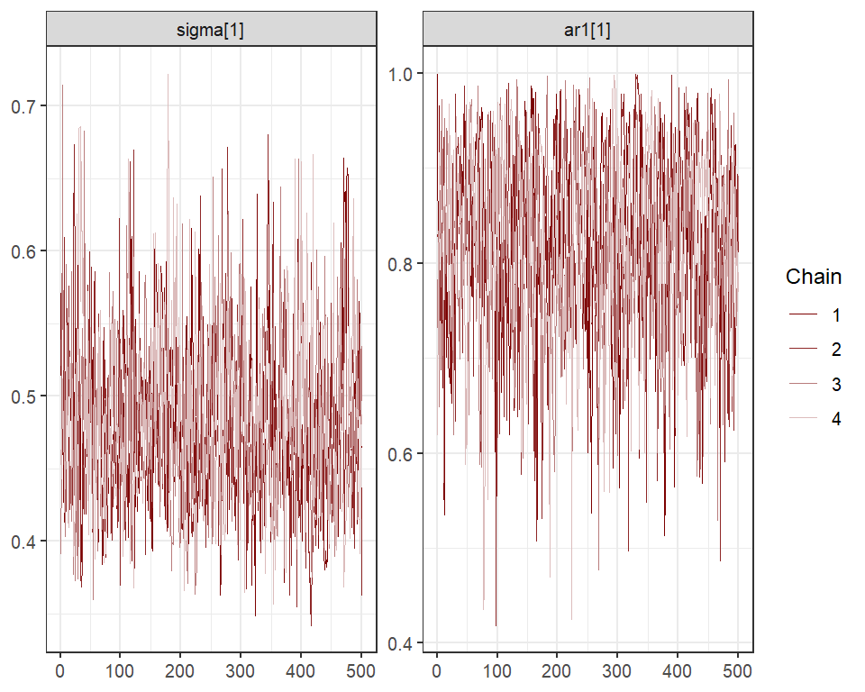
and for the latent trend parameters
mcmc_plot(lynx_mvgam, variable = 'trend_params', regex = TRUE, type = 'trace')
#> No divergences to plot.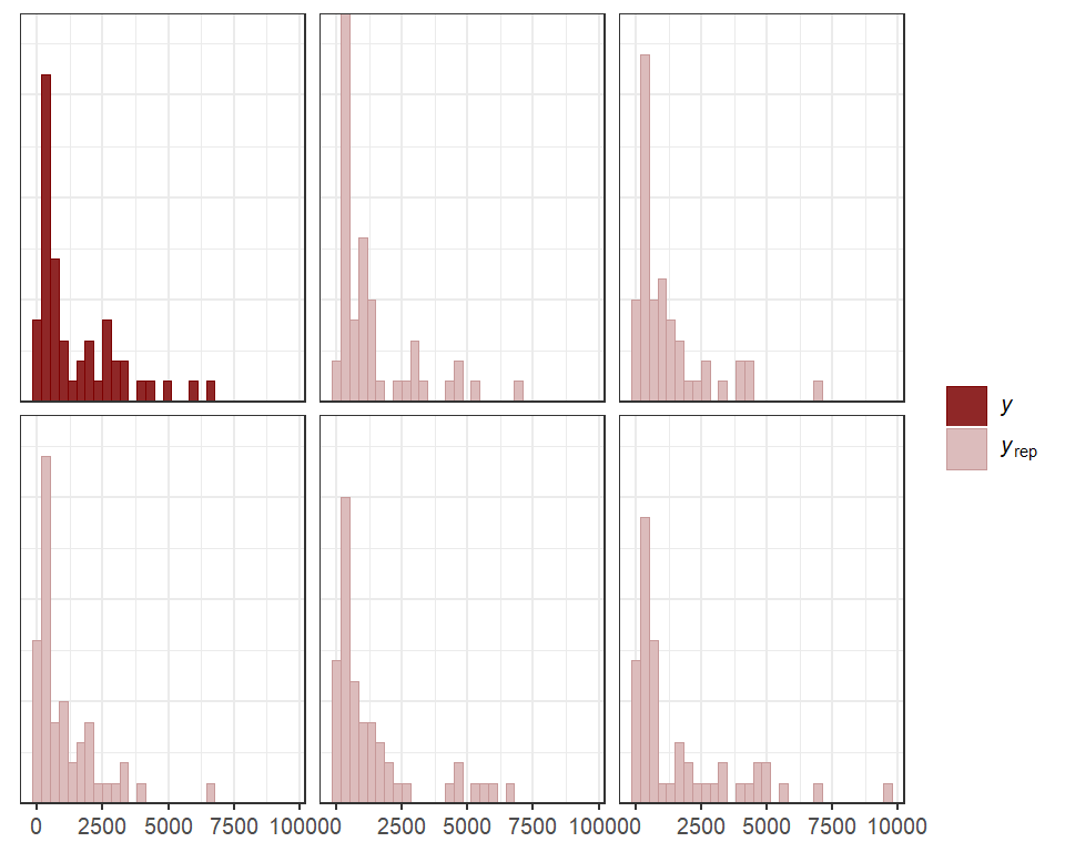
Use posterior predictive checks, which capitalize on the extensive functionality of the bayesplot package, to see if the model can simulate data that looks realistic and unbiased. First, examine histograms for posterior retrodictions (yhat) and compare to the histogram of the observations (y)
pp_check(lynx_mvgam, type = "hist", ndraws = 5)
#> `stat_bin()` using `bins = 30`. Pick better value with `binwidth`.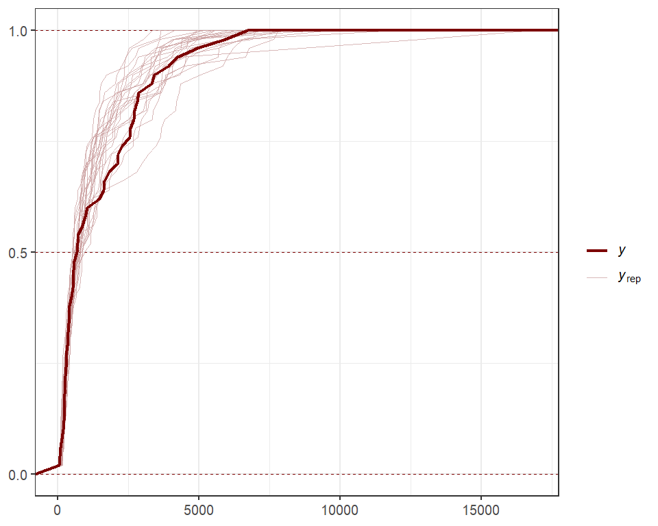
Next examine simulated empirical Cumulative Distribution Functions (CDF) for posterior predictions
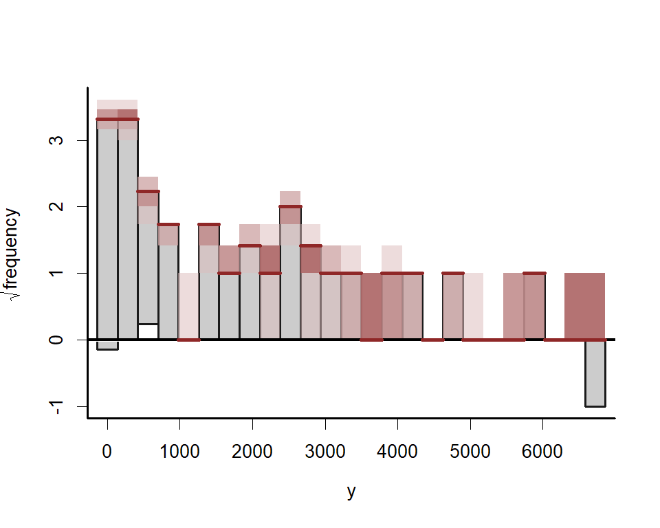
Rootograms are popular graphical tools for checking a discrete model’s ability to capture dispersion properties of the response variable. Posterior predictive hanging rootograms can be displayed using the ppc() function. In the plot below, we bin the unique observed values into 25 bins to prevent overplotting and help with interpretation. This plot compares the frequencies of observed vs predicted values for each bin. For example, if the gray bars (representing observed frequencies) tend to stretch below zero, this suggests the model’s simulations predict the values in that particular bin less frequently than they are observed in the data. A well-fitting model that can generate realistic simulated data will provide a rootogram in which the lower boundaries of the grey bars are generally near zero. For this plot we use the S3 function ppc.mvgam(), which is not as versatile as pp_check() but allows us to bin rootograms to avoid overplotting
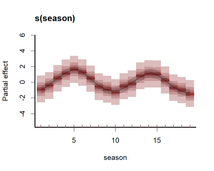
All plots indicate the model is well calibrated against the training data. Inspect the estimated cyclic smooth, which is shown as a ribbon plot of posterior empirical quantiles. We can also overlay posterior quantiles of partial residuals (shown in red), which represent the leftover variation that the model expects would remain if this smooth term was dropped but all other parameters remained unchanged. A strong pattern in the partial residuals suggests there would be strong patterns left unexplained in the model if we were to drop this term, giving us further confidence that this function is important in the model
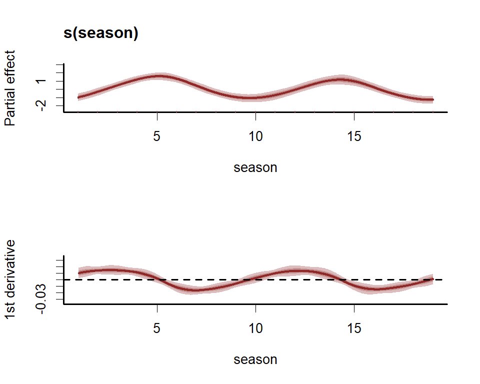
First derivatives of smooths can be plotted to inspect how the slope of the function changes. To plot these we use the more flexible plot_mvgam_smooth() function
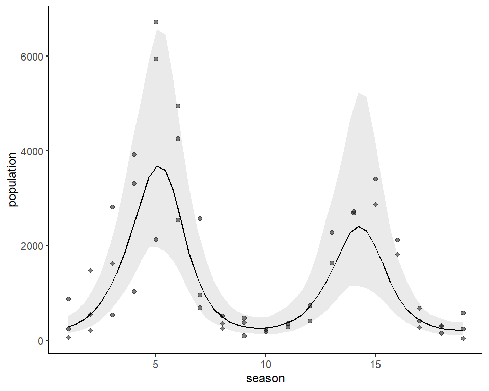
As for many types of regression models, it is often more useful to plot model effects on the outcome scale. mvgam has support for the wonderful marginaleffects package, allowing a wide variety of posterior contrasts, averages, conditional and marginal predictions to be calculated and plotted. Below is the conditional effect of season plotted on the outcome scale, for example:
require(ggplot2)
#> Loading required package: ggplot2
#> Warning: package 'ggplot2' was built under R version 4.3.3
plot_predictions(lynx_mvgam, condition = 'season', points = 0.5) +
  theme_classic()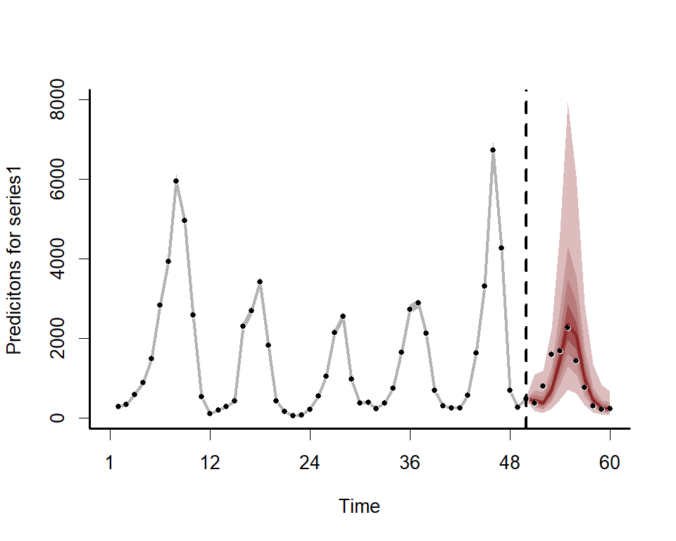
We can also view the mvgam’s posterior predictions for the entire series (testing and training)
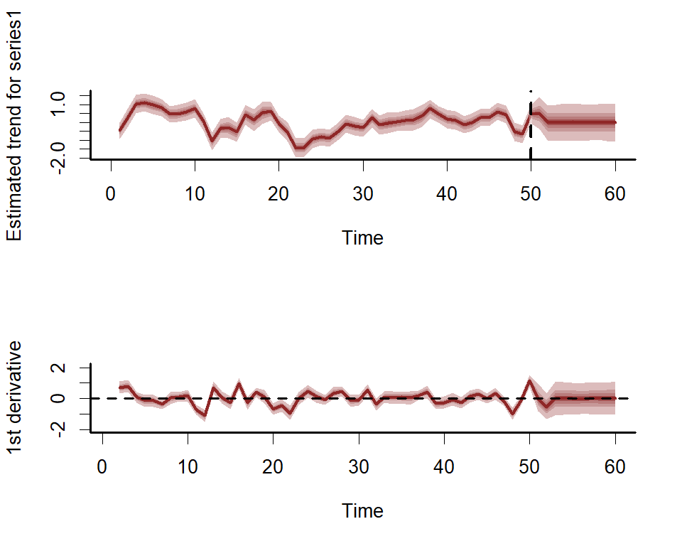
And the estimated latent trend component, again using the more flexible plot_mvgam_...() option to show first derivatives of the estimated trend
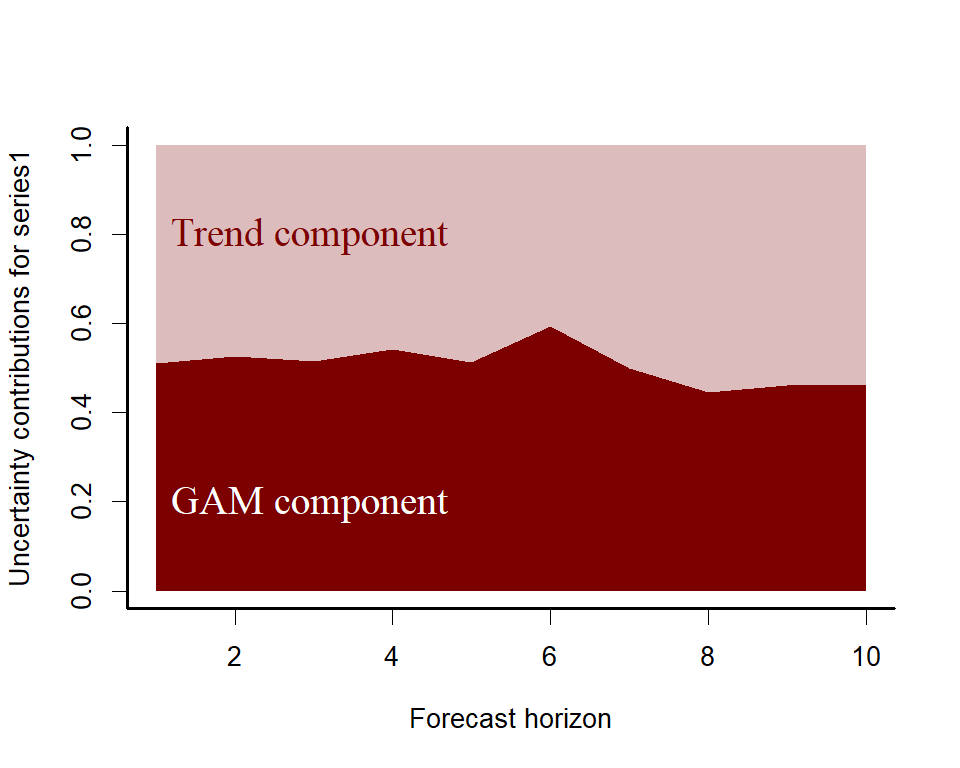
A key aspect of ecological forecasting is to understand how different components of a model contribute to forecast uncertainty. We can estimate relative contributions to forecast uncertainty for the GAM component and the latent trend component using mvgam
plot_mvgam_uncertainty(lynx_mvgam, newdata = lynx_test, legend_position = 'none')
text(1, 0.2, cex = 1.5, label="GAM component",
     pos = 4, col="white", family = 'serif')
text(1, 0.8, cex = 1.5, label="Trend component",
     pos = 4, col="#7C0000", family = 'serif')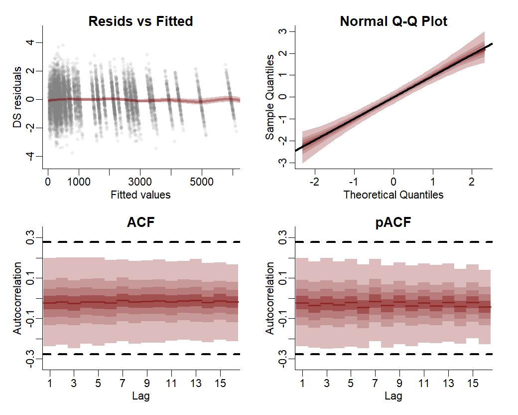
Both components contribute to forecast uncertainty. Diagnostics of the model can also be performed using mvgam. Have a look at the model’s residuals, which are posterior empirical quantiles of Dunn-Smyth randomised quantile residuals so should follow approximate normality. We are primarily looking for a lack of autocorrelation, which would suggest our AR3 model is appropriate for the latent trend
mvgam was originally designed to analyse and forecast non-negative integer-valued data. These data are traditionally challenging to analyse with existing time-series analysis packages. But further development of mvgam has resulted in support for a growing number of observation families. Currently, the package can handle data for the following:
gaussian() for real-valued datastudent_t() for heavy-tailed real-valued datalognormal() for non-negative real-valued dataGamma() for non-negative real-valued databetar() for proportional data on (0,1)bernoulli() for binary datapoisson() for count datanb() for overdispersed count databinomial() for count data with known number of trialsbeta_binomial() for overdispersed count data with known number of trialsnmix() for count data with imperfect detection (unknown number of trials)tweedie() for overdispersed count dataNote that only poisson(), nb(), and tweedie() are available if using JAGS. All families, apart from tweedie(), are supported if using Stan. See ??mvgam_families for more information. Below is a simple example for simulating and modelling proportional data with Beta observations over a set of seasonal series with independent Gaussian Process dynamic trends:
set.seed(100)
data <- sim_mvgam(family = betar(),
                  T = 80,
                  trend_model = 'GP',
                  prop_trend = 0.5,
                  seasonality = 'shared')
plot_mvgam_series(data = data$data_train, series = 'all')
mod <- mvgam(y ~ s(season, bs = 'cc', k = 7) +
               s(season, by = series, m = 1, k = 5),
             trend_model = 'GP',
             data = data$data_train,
             newdata = data$data_test,
             family = betar())
Inspect the summary to see that the posterior now also contains estimates for the Beta precision parameters \(\phi\). We can suppress a summary of the \(\beta\) coefficients, which is useful when there are many spline coefficients to report:
summary(mod, include_betas = FALSE)
#> GAM formula:
#> y ~ s(season, bs = "cc", k = 7) + s(season, by = series, m = 1,
#>     k = 5)
#>
#> Family:
#> beta
#>
#> Link function:
#> logit
#>
#> Trend model:
#> GP
#>
#> N series:
#> 3
#>
#> N timepoints:
#> 80
#>
#> Status:
#> Fitted using Stan
#> 4 chains, each with iter = 1000; warmup = 500; thin = 1
#> Total post-warmup draws = 2000
#>
#>
#> Observation precision parameter estimates:
#>        2.5% 50% 97.5% Rhat n_eff
#> phi[1]  5.5 8.4    12    1  1516
#> phi[2]  5.8 8.7    13    1  1333
#> phi[3]  5.6 8.5    12    1  1690
#>
#> GAM coefficient (beta) estimates:
#>              2.5%  50% 97.5% Rhat n_eff
#> (Intercept) -0.19 0.19  0.44    1   822
#>
#> Approximate significance of GAM smooths:
#>                            edf Ref.df Chi.sq p-value
#> s(season)                4.639      5  35.50  <2e-16 ***
#> s(season):seriesseries_1 0.887      4   0.53    0.98
#> s(season):seriesseries_2 0.940      4   0.44    0.99
#> s(season):seriesseries_3 1.391      4   1.40    0.78
#> ---
#> Signif. codes:  0 '***' 0.001 '**' 0.01 '*' 0.05 '.' 0.1 ' ' 1
#>
#> Latent trend marginal deviation (alpha) and length scale (rho) estimates:
#>             2.5%  50% 97.5% Rhat n_eff
#> alpha_gp[1] 0.10 0.44  0.98 1.00   770
#> alpha_gp[2] 0.37 0.74  1.30 1.00  1129
#> alpha_gp[3] 0.16 0.46  0.98 1.00   824
#> rho_gp[1]   1.20 3.80 14.00 1.00   705
#> rho_gp[2]   1.80 7.30 33.00 1.01   411
#> rho_gp[3]   1.30 4.90 23.00 1.01   658
#>
#> Stan MCMC diagnostics:
#> n_eff / iter looks reasonable for all parameters
#> Rhat looks reasonable for all parameters
#> 3 of 2000 iterations ended with a divergence (0.15%)
#>  *Try running with larger adapt_delta to remove the divergences
#> 0 of 2000 iterations saturated the maximum tree depth of 12 (0%)
#> E-FMI indicated no pathological behavior
#>
#> Samples were drawn using NUTS(diag_e) at Wed May 08 9:38:56 AM 2024.
#> For each parameter, n_eff is a crude measure of effective sample size,
#> and Rhat is the potential scale reduction factor on split MCMC chains
#> (at convergence, Rhat = 1)
Plot the hindcast and forecast distributions for each series
layout(matrix(1:4, nrow = 2, byrow = TRUE))
for(i in 1:3){
  plot(mod, type = 'forecast', series = i)
}
There are many more extended uses of mvgam, including the ability to fit hierarchical GAMs that include dynamic coefficient models, dynamic factor and Vector Autoregressive processes. See the package documentation for more details. The package can also be used to generate all necessary data structures, initial value functions and modelling code necessary to fit DGAMs using Stan or JAGS. This can be helpful if users wish to make changes to the model to better suit their own bespoke research / analysis goals. The following resources can be helpful to troubleshoot:
This project is licensed under an MIT open source license
I’m actively seeking PhD students and other researchers to work in the areas of ecological forecasting, multivariate model evaluation and development of mvgam. Please reach out if you are interested (n.clark’at’uq.edu.au)